Integral Equations and the Method of Green's Functions

This is an evaluated Mathematica notebook. If you have Mathematica or MathReader (which is available free from WRI, you may download the notebook file. This notebook contains some Mathematica calculations for chapter I (Green track) of Harrell and Herod's WWW textbook.

To execute this Mathematica notebook, you need to put the cursor in the calculation cells in order and push return. You may find it instructive to modify the inputs and see what results.

Let's consider the integral equation

y(x) = K y + f(x)
where K g denotes the integral from 0 to x of Sin[Pi(x-t)] g(t) dt, we take f(x) = x, and the variable x runs from 0 to 1.

This kernel is not separable, even though a trigonometric identity can be used to write Sin[Pi(x-t)] as a sum in the form a_p(x) b_p(t), because the limits of the integral depend on x. (The equation is said to be of Volterra type.)

We first ask whether this integral kernel is small in the two senses we have learned about. This means checking whether either of two calculations is less than 1. Notice that since the integral runs only from 0 to x, the integral kernel is
K(x,t) = Sin[Pi(x-t)] , 0 < t < x < 1
K(x,t) = 0 , 0 < x < t < 1
The integrals we shall calculate will thus only run from 0 to x in the variable t.

To see if the kernel is small in the sense appropriate for a continuous solution y(x), we calculate:

In[1]:=

  Integrate[Sin[Pi(x-t)], {t,0,x}]

Out[1]=

  1    Cos[Pi x]
  -- - ---------
  Pi      Pi

This is maximized by 2/š, which is less than 1:

In[2]:=

  N[2/Pi]

Out[2]=

  0.63662

We are thus guaranteed that the integral equation has a continuous solution, and that we can calculate it by iteration.

To see if the kernel is small in the sense appropriate for a square-integrable solution y(x), we calculate:

In[3]:=

  Integrate[Sin[Pi(x-t)]^2, {t,0,x}]

Out[3]=

  -(-2 Pi x + Sin[2 Pi x])
  ------------------------
            4 Pi

In[4]:=

  Integrate[%, {x,0,1}]

Out[4]=

                  2
   -1     1 + 2 Pi
  ----- + ---------
      2         2
  8 Pi      8 Pi

In[5]:=

  N[%]

Out[5]=

  0.25

This is also less than 1, so we are guaranteed that iteration will lead us to the solution in the r.m.s. sense. Normally this is a weaker statement than the previous one, so we are not surprised.

Now let's calculate the solution

In[6]:=

  Clear[K]

In[7]:=

  K[f_] := Integrate[Sin[Pi(x-t)] (f /. x -> t), {t,0,x}]

The obscure command embedded in this, (f /. x -> t), has the effect of changing the variable in the function f from x to t, which we need to do to integrate properly.

In[8]:=

  y1[x_] = K[x]

Out[8]=

  x    Sin[Pi x]
  -- - ---------
  Pi        2
          Pi

In[9]:=

  y2[x_] = K[y1[x]]

Out[9]=

  4 Pi x + 2 Pi x Cos[Pi x] - Sin[Pi x]   5 Sin[Pi x]
  ------------------------------------- - -----------
                      3                          3
                  4 Pi                       4 Pi

In[10]:=

  y3[x_] = K[y2[x]]

Out[10]=

  -23 Sin[Pi x]
  ------------- + (16 Pi x + 14 Pi x Cos[Pi x] - 
          4
     16 Pi
   
                         2  2                    4
       7 Sin[Pi x] + 2 Pi  x  Sin[Pi x]) / (16 Pi )

In[11]:=

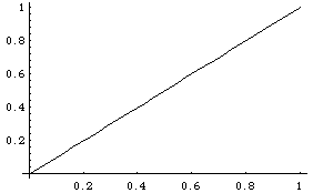
  {Plot[x, {x,0,1}], Plot[y1[x]+x, {x,0,1}], \
      Plot[y2[x]+y1[x]+x, {x,0,1}], \
      Plot[y3[x]+y2[x]+y1[x]+x, {x,0,1}]}

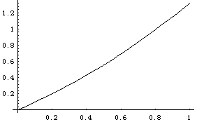
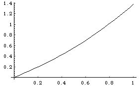
Out[12]=

  {-Graphics-, -Graphics-, -Graphics-, -Graphics-}

These last two plots look somewhat similar, which is an indication that we are getting close to the exact solution. How far away are we? Well, if you stop the series at third order,

f + Kf + K² f + K³ f,
then the error is K⁴ f + K⁵ f +...

We know that the calculations we must check for convergence are actually bounds
of the form ||K g|| <= c || g||,
where for the infinity norm (for continuous functions), c = 2/ \pi, and for the r.m.s. norm (for square-integrable functions) c = 1/2. (The calculation we did gave 1/4, but that is actually c²).

The right scale for this problem is ||x||_infinity = 1 or, respectively, ||x||₂ = 1/Sqrt[3]

In[13]:=

  N[1/Sqrt[3]]

Out[13]=

  0.57735

The norm of Kⁿ f is at most cⁿ times the norm of f (either norm), so the size of the error is
c⁴ + c⁵ + ... = c⁴ (1 + c + c² + ...) = c⁴/(1-c).

Conclusion: The maximum possible error
|x+y₁+y₂+y₃ - y_exact(x)|
is at most

In[14]:=

  N[(2/Pi)^4 /(1-2/Pi)]

Out[14]=

  0.452022

The maximum possible error in the rms sense is

In[15]:=

  (1/2)^4 / (1-1/2)

Out[15]=

  1
  -
  8

Which is fairly small. If we want more accuracy, we need more terms. With 8 terms,

In[16]:=

  N[(2/Pi)^8 /(1-2/Pi)]

Out[16]=

  0.0742471

In[17]:=

  N[(1/2)^7]

Out[17]=

  0.0078125

So we would be within 5% uniformly and about 1% in the rms sense. Actually, we are probably doing much better, for already at third order,

In[18]:=

  Plot[y3[x], {x,0,1/2}]
  Plot[y3[x], {x,1/2,1}]

Out[19]=

  -Graphics-

Out[20]=

  -Graphics-

In[21]:=

  y4[x_] = K[y3[x]]
  y5[x_] = K[y4[x]]
  y6[x_] = K[y5[x]]
  y7[x_] = K[y6[x]]
  y8[x_] = K[y7[x]]

Out[21]=

  -51 Sin[Pi x]
  ------------- + (96 Pi x + 114 Pi x Cos[Pi x] - 
          5
     32 Pi
   
           3  3                                 2  2
       2 Pi  x  Cos[Pi x] - 57 Sin[Pi x] + 24 Pi  x  Sin[Pi x]
   
                 5
       ) / (96 Pi )

Out[22]=

  -443 Sin[Pi x]
  -------------- + (768 Pi x + 1122 Pi x Cos[Pi x] - 
           6
     256 Pi
   
            3  3
       36 Pi  x  Cos[Pi x] - 561 Sin[Pi x] + 
   
             2  2                 4  4                     6
       282 Pi  x  Sin[Pi x] - 2 Pi  x  Sin[Pi x]) / (768 Pi )

Out[23]=

  -949 Sin[Pi x]
  -------------- + (7680 Pi x + 13110 Pi x Cos[Pi x] - 
           7
     512 Pi
   
             3  3                 5  5
       570 Pi  x  Cos[Pi x] + 2 Pi  x  Cos[Pi x] - 
   
                               2  2
       6555 Sin[Pi x] + 3660 Pi  x  Sin[Pi x] - 
   
            4  4                      7
       50 Pi  x  Sin[Pi x]) / (7680 Pi )

Out[24]=

  -4027 Sin[Pi x]
  --------------- + (92160 Pi x + 178110 Pi x Cos[Pi x] - 
            8
     2048 Pi
   
              3  3                  5  5
       9360 Pi  x  Cos[Pi x] + 66 Pi  x  Cos[Pi x] - 
   
                                 2  2
       89055 Sin[Pi x] + 53370 Pi  x  Sin[Pi x] - 
   
              4  4                 6  6
       1020 Pi  x  Sin[Pi x] + 2 Pi  x  Sin[Pi x]) / 
   
              8
     (92160 Pi )

Out[25]=

  -8483 Sin[Pi x]
  --------------- + (1290240 Pi x + 2763810 Pi x Cos[Pi x] - 
            9
     4096 Pi
   
                3  3                    5  5
       165690 Pi  x  Cos[Pi x] + 1680 Pi  x  Cos[Pi x] - 
   
           7  7
       2 Pi  x  Cos[Pi x] - 1381905 Sin[Pi x] + 
   
                2  2                     4  4
       871920 Pi  x  Sin[Pi x] - 20580 Pi  x  Sin[Pi x] + 
   
            6  6                         9
       84 Pi  x  Sin[Pi x]) / (1290240 Pi )

What beautiful functions! How would you like to calculate them by hand?

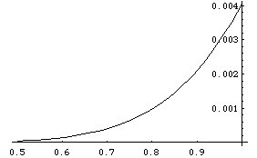
You can hardly see the difference between the really accurate solution and the third order solution:

In[26]:=

  Plot[{x+y1[x]+y2[x]+y3[x]+y4[x]+y5[x]+y6[x] \
      + y7[x]+y8[x], \
       x+y1[x]+y2[x]+y3[x]},    {x,0,1}]

Out[27]=

  -Graphics-

In[28]:=

  Plot[{x+y1[x]+y2[x]+y3[x]+y4[x]+y5[x]+y6[x] \
      + y7[x]+y8[x], \
       x+y1[x]+y2[x]+y3[x]},    {x,.99,1}]

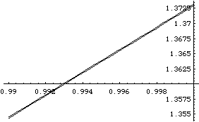
Out[29]=

-Graphics-

Up to chapter 5

Return to Table of Contents

Return to Evans Harrell's home page