Web page maintained by Evans M. Harrell, II, harrell@math.gatech.edu.
We begin with a first order partial differential equation:
1 F([[partialdiff]]u,[[partialdiff]]x) + 2 F([[partialdiff]]u,[[partialdiff]]y) = - 3 u(x,y) with u(0,y) = exp(- y^2). (1.1)
The equation is called first order because the partial derivatives are only of order one. There are no second order partials in equation (1.1).
The function u that satisfies this differential equation is a real number valued function u(x,y). It has partial derivatives in x and y and they are related by equation (1.1). Early in these notes, methods to solve this equation and to visualize the surface u(x,y) as a graph in R^3 will be developed.
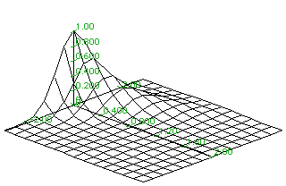
Here is the solution to this equation:
u(x,y) = exp(-3 x) exp(- [y-2 x]^2 ) (1.2)
There is no reason that you should know already that this is the solution. But, you can check to see that it is. Indeed, you should check that this is a solution for equation (1.1). The Maple syntax for drawing this figure is
> plot3d(exp(-3*x)*exp(-(y-2*x)^2), x=0..2, y=-3..3,
orientation=[-45,45], axes = NORMAL):

FIGURE 1.1 : Solutions for (1.1).
Figure 1.1 is the graph of the solution. How could one have guessed that the graph might have that appearance? Having that exponential distribution as the initial value along the line x = 0 suggested the spike and dampening above that line, where u(0,y) = exp(-y^2). Recalling that in ordinary differential equations, the solutions of
F(dz,dx) = - 3 z(x)
decay in the x direction. This suggest that solutions for (1.1) will dampen to zero as x increases. Thus, some quantitative geometric ideas are suggested by just the form of the equation and, also, by some sophistication of the reader.
There are at least three ways to conceive of developing a mathemat-ical structure for understanding solutions for (1.1): numerically, analyti-cally, and conceptually in a space of functions. To think of u as satisfying a differential equation and of solving for u numerically is the subject of other courses. That method involves creating a mesh over the plane and thinking of making one step in the x direction and filling in a new line in the y direction, using the interdependent relationship between how u changes in x and y. The function space ideas are rich and have, historically, been the subject of much attention. Often, in that context, one rewrites the partial differential equation as an ordinary differential equation in an appropriate function space. This course, on the other hand, will develop analytic methods to solve some types of partial differential equations. We will attempt to find solutions in closed form such as (1.2) is a solution for (1.1). Just as sophomore differential equations introduced ordinary differential equations and gave some simple first ideas of how ordinary differential equations are solved, so these notes will do this for partial differential equations. It is certainly not expected that the methods are exhaustive. We do not propose to present methods to solve all partial differential equations!
Here is a geometric idea for how the methods of this course will work. We will construct graphs of solutions u. We will need to agree to take the positive, horizontal axis as the x axis; the vertical axis will be the y axis, as usual. At the outset, we consider the right half-plane as being swept out by the y-axis moving continuously to the right at varying speeds, stretching and deforming as it evolves. The method of solving the partial differential equation of the next sections can be conceived of intuitively in this manner: given an initial u(0,y) graphed over the y axis, follow that graph as it remains over the evolving y axis sweeping out the right half plane. Just as the y axis expands and contracts as it moves to the right, so the initial graph of u changes. We could think of the shape of the graph being given by u(x,y). The nature of the motion of the y axis moving to the right is critical, as well as how u deforms as it follows along above that evolving y axis.
The notion of "sweeping out the right half-plane" is only intutive. This must be described analytically to solidify the idea. We begin making these ideas precise in this section. In the next section, we make connections with how u changes as x increase and y evolves.
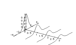
We have included in these notes some of the Maple syntax used to draw figures and to work Examples. Solutions for the Exercises can be made by using the syntax. For example, Maple could be used to draw the following figure:

FIGURE 1.2
> with(plots):
> spacecurve({[0,t,exp(-t^2)],[1,t,exp(-t^2)/2],
[2,t,exp(-t^2)/3],[3,t,exp(-t^2)/4]}, t=-4..4,
orientation=[-55,45],axes=NORMAL);
Figure 1.2 illustrates how the initial distribution moves through the right half plane, and it evolves to produce the surface such as shown as Figure 1.1.
We keep up with this evolving y axis with a pair of differential equations:
A(F(dx,dt) = p(x(t), y(t)), x(0) = 0,F(dy,dt) = q(x(t), y(t)), y(0) = [[eta]].) (1.3)
These equations make an analytic model to simulate the motion in the positive x direction and keep track of the contractions and expansions of the y axis as it moves to the right in time.
The possibilities for what can happen are so innumerable as to be chaotic. We need to make some sense of what can be expected. Here are some simple ideas.
It would be best if x(t) is increasing for then, as the y axis sweeps through the right-half plane, it will be a continuously advancing image. If p(x,y) in equation (1.3) were the constant 1, the motion would be simple for the y axis would progress to the right in an orderly manner: linearly, and at a uniform rate in time. Probably this is too restrictive an idea. One might think of the y axis as hanging back in some spots and surging forward in others. To achieve the goal that the y axis should sweep steadfastly to the right through the right-half plane, we ask that p(x,y) should be positive for all x and y.
At this beginning, we ask that for every point {x,y} in the right-half plane, the equations (1.3) determine the direction of motion forward. That is, p(x,y) and q(x,y) should be sufficiently ordinary so that solutions can be found for all t > 0.
There is another idea that is important. If a point {a,b} is chosen in the right-half plane, it would be desirable to know enough about the trajectories that started from the y axis sweeping forward as x and y evolve so that, with certainty, there is exactly one {0,[[eta]]} on the y-axis at which a trajectory started and moved to {a,b}. Moreover, that trajectory arrived at {a,b} at exactly one time t. It may be that determining the [[eta]] and the t will be difficult, but that makes the problem interesting! One way of thinking of this is: Given a and b, can the equations for x(t) and y(t) be "inverted" to find y(0) and t as functions of a and b?
If the answer to that question is yes, then given a and b, you can tell where the trajectory started which arrived at {a,b} and for what "t" it arrived there.
These ideas are at the core of solving partial differential equations by the methods of characteristics. The trajectories {x(t), y(t)} are the characteristics of the equation. We will find that the solutions "flow" along the characteristics in a rather simple manner. For this reason, a little attention needs to be paid to this geometric idea at the beginning.
A summary of what to expect in the equations (1.3) would go like this:
(a) p(x,y) > 0 for all x > 0 and all y;
(b) solutions for (1.3) exist for all t > 0; and
(c) if x(t) and y(t) are solutions for (1.3) and {a,b} is in the right half-plane, then the equations
x(t) = a
y(t) = b,
can be inverted to solve for t and [[eta]].
Each of these ideas has a geometric interpretation that should be understood.
EXAMPLE 1: Suppose that p(x,y) = 1 and q(x,y) = 1, for x > 0. Find {x(t), y(t)} so that
F(dx,dt) = 1, x(0) = 0,
F(dy,dt) = 1, y(0) = [[eta]].
Solutions are x(t) = t and y(t) = t+[[eta]]. We solve for [[eta]] and t in terms of x and y.
The inversion for this example is easy:
[[eta]](x,y) = y - x and t(x,y) = x.
One could speak of the results this way: Pick a point {a,b}. It can be determined where to start, [[eta]] = b - a, so that following the trajectory of the associated differential equation gets you to {a,b} at time t = a.
EXAMPLE 2: The following example is a little more interesting. Let p(x,y) = 1 and q(x,y) = (2-y) y for x > 0 and y > 0. The function x(t) = t as before. You may recall how to solve for y. Here is Maple syntax for obtaining the solution:
> dsolve({D(y)(t)=(2-y(t))*y(t), y(0) = eta},y(t));
Solutions y are
y(t) = F(2 [[eta]],[[eta]] + e ^-2t (2 - [[eta]]))
We consider the problem of inversion. That is, given a and b, can we find [[eta]] and t so that if y(0) = [[eta]] then {x(t), y(t)} = {a,b}? To find t is easy: t = a. To solve
F(2 [[eta]],[[eta]] + e ^-2t (2 - [[eta]])) = b
for [[eta]] is more interesting. Maple provides a solution.
> solve(y(t)=b,eta);
[[eta]] = F(2 b e^-2t,2 + b (e^-2t - 1)).
The equation
y[[minute]] = (2 - y).y
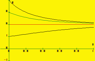
in y is called a Ricatti equation. You might look back for this type equation in your undergraduate differential equation text. It is interesting to analyze how the graph must look. Maple draws the graph, too. The graph is Figure 1.3.
> y1(t):=subs(eta=1,y(t)); y2(t):=subs(eta=2,y(t));
y3(t):=subs(eta=3,y(t)); y4(t):=subs(eta=4,y(t));
> plot({[t,y1(t),t=0..1],[t,y2(t),t=0..1],[t,y3(t),t=0..1],
[t,y4(t),t=0..1]},t=-.1..1,y=-1..4);
Before these notes are finished, we will relax the conditions we have described a little. We will find that "flows" can come to a point from different initial points. One can think of this as having information coming from two sources. Not to worry; we can determine how u should behave at the point {a,b}, anyway.

Figure 1.3 : Plots for Example 2.
Exercises
1.1. Verify that equation (1.2) describes a solution for (1.1).
1.2. Find x and y to solve (1.3), invert them to solve for t and y(0) = c as functions of x and y, and draw the curves characteristic of the flow for each of the following:
a. p(x,y) = x+2, q(x,y) = 2y, [[eta]] > 0.
b. p(x,y) = 1, q(x,y) = 1-y, [[eta]] > 0.
c. p(x,y) = 4, q(x,y) = x+2y, [[eta]] > 0.
d. p(x,y) = 3x + 4y, q(x,y) = -x -2y, [[eta]] > 0. (Hint: solve x(t) = a, y(t) = b for t and [[eta]] with a computer algebra system.)
1.3. Pathological Examples:
a. Consider two examples: in both p(x,y) = 1. For one, q(x,y) = y^2 and for the other, q(x,y) = 1+y^2. Try starting y(0) = 1. In the first case, y(t) = 1/(1-t) and in the second, y(t) = tan(t+[[pi]]/4). In both cases, x(t) = t. Verify that these are solutions for x[[minute]] = p(x,y) and y[[minute]] = q(x,y). Draw the trajectories. This is clearly an unsatisfactory state of affairs to achieve the kind of geometry we were considering.
b. Take p(x,y) = 1 for all x and y and q(x,y) = - sgn(y), where sgn(y) = 1 if y > 0, -1 if y < 0 and 0 if y = 0. For each {a,0}, a > 0, there are an infinity of numbers [[eta]] such that the solutions that start at {0,[[eta]]} arrive at {a,0} at some time.