Linear Methods of Applied Mathematics

Evans M. Harrell II and James V. Herod*

*(c) Copyright 1994,1995,1996 by Evans M. Harrell II and James V. Herod. All rights reserved.

XIII. Solving Y = KY + f

In this chapter we shall learn how to solve integral equations in three situations:

• K has a separable kernel,

• K has norm less than one,

• K is approximated by K's with separable kernels.

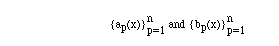
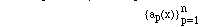
First we suppose that there are an integer n and functions

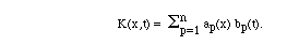
such that, for each p , a_p and b_p are in L²[0,1]. Then K has a separable kernel if its kernel is given by

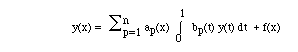
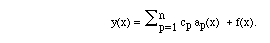
With the supposition the K is separable, it is not hard to find y such that y = Ky + f, for this equation can be re-written as

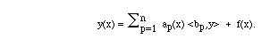
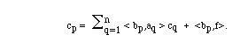
or, using the notation of inner products,

One can guess that, if the sequence

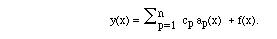
of functions on [0,1] is a linearly independent sequence, then y will have this special form:

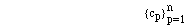
there is a sequence {cp} of numbers such that

In fact, supposing there is such a sequence, we determine what it should be.

Suppose

Substitute this in the equation to be solved:

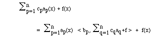
and we see that

This now reduces to a matrx problem:

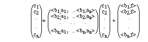
Define K and f to be the matrix and vector so defined that the last equation is rewritten as

       c = K c + f.

We now employ ideas from linear algebra. The equation c = K c + f has exactly one solution provided

det( 1 - K ) != 0.

The Fredholm Alternative Theorems for matrices address these ideas. (Review the alternative theorems for matrices.) If the sequence

is found then we have a formula for y(x).

EXAMPLE: In Exercises 1.2, it should have been established that if

       K(x,t) = 1 + sin([[pi]]x) cos([[pi]]t),

then

       K*(x,t) = 1 + sin([[pi]]t) cos([[pi]]x).

Also,

        y = Ky has solution y(x) = 1

and

       y = K*y has solution y(x) = [[pi]] + 2 cos([[pi]]x).

It is the promise of the Fredholm Alternative theorems that

       y = Ky + f

has a solution provided that

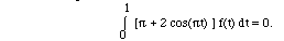
Let us try to solve y = Ky + f and watch to see where the requirement that f should be perpendicular to the function [[pi]] +2 cos([[pi]]t) appears.

To solve y = Ky + f is to solve

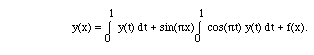
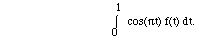
We guess that the solution is of the form y(x) = a + b sin([[pi]]x) + f(x) and substitute this for y:

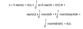
From this, we get the algebraic equations

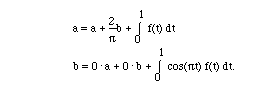
Hence, in our guess for y, we find that a can be anything and that b must be

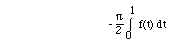
and also must be

The naive pupil might think this means there are two (possibily contradictory) requirements on b. The third of the Fredholm Alternative theorems assures the student that there is only one requirement!

Take [[phi]]₀(x) to be f(x) and [[phi]]₁ to be defined by

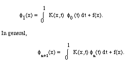
It is reasonable to ask: does this generated sequence converge to a limit and in what sense does it converge? The answer to both questions can be found under appropriate hypothesis on K.

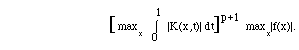
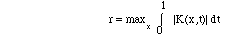
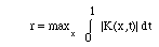
THEOREM If K satisfies the condition that

then limp [[phi]]_p(x) exists and the convergence is uniform on [0,1] - in the sense that if u = lim_p[[phi]]_p then

       lim_p max_x | u(x) - [[phi]]_p(x) | = 0.

SUGGESTION FOR PROOF: Note that

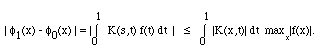
Furthermore, if p is a positive integer, the distance between successive iterates can be computed:

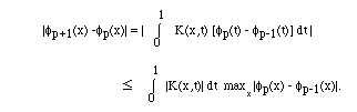
Inductively, this does not exceed

Thus, if

and n > m then

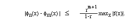
Hence, the sequence {[[phi]]_p} of functions converges uniformly on [0,1] to a limit function and this limit provides a solution to the equation

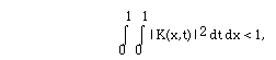
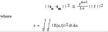
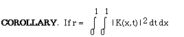
COROLLARY. If

and

       u = lim_p [[phi]]_p

then

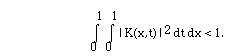
THEOREM If K satisfies the condition that

then lim_p [[phi]]p(x) exists and the convergence is in norm- meaning that if u = lim_p[[phi]]p then

       lim_p || u(x) - [[phi]]p(x) || = 0.

INDICATION OF PROOF. The analysis of the nature of the convergence will go like this:

       || [[phi]]1 - [[phi]]0 || ²

is defined to be

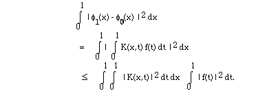
As before,

and

       u = lim_p [[phi]]p

then

       ||u - [[phi]]m || < F(r^m+1,1 - r) ||f||.

THE RESOLVENT.

Before addressing the final case - where

       K does not have a separable kernel,

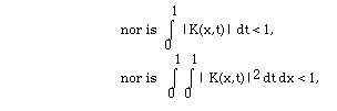
we generate "resolvents" for the integral equations.

Re-examining the iteration process:

    [[phi]]₀(x) = f(x),

    [[phi]]₁(x) = K[[phi]]₀(x) + f(x)

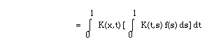
    [[phi]]₂(x) = K(K([[phi]]₀))x + K(f)(x) + f(x)

One writes [[phi]]₀=f, [[phi]]₁=Kf+f, [[phi]]₂ = K[Kf+f] + f = K²f+Kf+f, .....

In fact, with

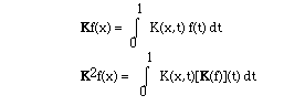
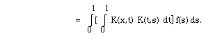
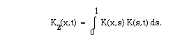
Hence, the kernel K₂ associated with K² is

Inductively,

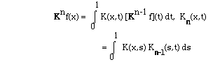
and

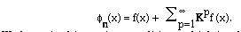
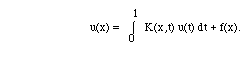
We have, in this section, conditions which imply that

       [[Sigma]]p=1 K^pf

converges and that its limit y satisfies y = Ky + f. Many authors call this series of operators the "resolvent" and denote

       R = [[Sigma]]p=1 K^p.

Note that R is a function which operates on elements of L²[0,1]. One writes that

      y = Ky + f

has solution

       y(x) = [( 1 + R ) f](x) = f(x) + I(0,1, ) R(x,t) f(t) dt.

Suggestive algebra can be made by identifying (1 + R ) as

      (1 - K ) ^-1 = 1 + K( 1 - K ) ^-1, so that R = K ( 1 - K ) ^-1.

Please refer to the accompanying Mathematica notebook for the solution by iteration of a typical integral equation, including error estimates.

Continue with this chapter

Return to Table of Contents

Return to Evans Harrell's home page