Web page maintained by Evans M. Harrell, II, harrell@math.gatech.edu.
Seems these always come up late in the quarter and are dismissed in a string of series and a flurry of finishing the quarter. Series are introduced as a technique for solving ordinary differential equations in undergraduate courses. Always, there are accompanying questions of when then series converges and there are hopes of finding recurrence formulas for the coefficients.
Surely, the existence of these computer algebra systems can relieve some of the tediousness of this study.
There are two ordinary differential equations that we consider for the purposes of this section. Actually, there is an infinity of Bessel's functions, but we must not get lost in the generality that is available. Consider these two:
0 = (rR')' + rR = rR'' + R' + rR
and
0 = (rR')' + rR - R/r = rR'' + R' + (r-1/r)R.
More often these are written as
0 = r2 R'' + rR + r2R and 0 = r2 R'' + rR + (r2-1) R.
Recalling the tools of series, one uses the methods of Frobenius to solve these equations. The student can look in the index of any text in partial differential equations or ordinary differential equation and find, not only methods to determine the series solutions for these equations, but also relations about the two equations. One is reminded that because the ordinary differential equations above are second order, it is expected that there are two linearly independent solutions to each. One of the two is bounded at zero and the other goes unbounded at zero. These are typically called the Bessel functions of the first and second kind respectively.
What is suggested here is in the context of using computer algebra systems to see the properties. For that purpose, note that MAPLE calls the Bessel function of the first kind BesselJ(0,x). BesselY(0,x) is the unbounded solutions for the first equation. Humans denote these J0(x) and Y0(x). For the second equation, BesselJ(1,x) = J1(x) and BesselY(1,x) = Y1(x). As typical, choices on the solutions are determined by boundary or initial conditions. The second kind solutions are most typically dismissed because they are unbounded at zero.
Here is a way to get the series expansions for J0(x) and J1(x) about x = 0:
* series(BesselJ(0,x),x=0,8);series(BesselJ(1,x),x=0,8);
2 4 6 8
1 - 1/4 x + 1/64 x - 1/2304 x + O(x )
3 5 7 8
1/2 x - 1/16 x + 1/384 x - 1/18432 x + O(x )
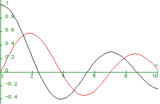
Here are their graphs and the MAPLE syntax to graph them.
* plot({BesselJ(0,x),BesselJ(1,x)},x=0..10);
Figure 20.1
One should note that J0 and J1 have an infinity of zeros and that these "intertwine" much as the cosine and sine do. Indeed, J0(0) = 1, J1(0)= 0. Don't push the comparison with sine and cosine too far: these functions are not periodic!
One more note: J0'(x) = - J1(x) and (x J1(x))' = x J0(x).
Now, here is the application to a partial differential equation. Suppose that {a,b} is a point in the plane and let F(s) be a real function. Form the composition
s = 2 R((x-a)(y-b))
u(x,y) = F(s) = F(2 R((x-a)(y-b)) ).
Then ux,y + u = 0 provided F satisfies the differential equation
0 = Fss + F(Fs,s) + F.
That is, a composition of a Bessel's equation of the first kind provides a solution to this elusive PDE:
Ux,y + U = 0.
Other solutions are sin(x+y) and cos(x+y).
Exercises:
1. Make and graph solutions for
uxy - u = 0.
2. Show that u(x,y) = 1 - BesselJ(0,x) satisfies uxy - u = 1. Plot the graph on [0,7]x[0,7].
Work in Progress: Make examples and exercises to connect this with the next section.