Web page maintained by Evans M. Harrell, II, harrell@math.gatech.edu.
F([[partialdiff]]2w,[[partialdiff]]x2) - F([[partialdiff]]2w,[[partialdiff]]y2) + d wx + e wy + f w = 0.
We know that the characteristics are y = +/- x and these characteristics change the equation to
uxy + a ux + b uy + c u = 0. (23.1)
Define the left side to be L[u], so that
L[u] = uxy + a ux + b uy + c u. (23.2)
If v is a twice differentiable function then
vuxy - vxyu = (vux)y - (vyu)x,
vaux = (vau)x - (va)x u, (23.3)
and vbuy = (vbu)y - (vb)y u.
If M[v] = vxy - (va)x - (vb)y + cv,
U = vau - vy u, (23.4)
and V = vbu + vux
Then, we argue that v L[u] - M[v] u = Ux + Vy (23.5)
as follows:
vL[u] - M[v] u =
= (vuxy + vaux + vbuy + vcu) - (vxy u - (va)xu - (vb)yu + vcu)
= (vux)y - (vyu)x + (vau)x + (vbu)y
= Ux + Vy
By Green's Theorem, or Stokes' Theorem as presented in these notes,
òòD [v L[u] - M[v] u] dx dy = òòD [Ux + Vy] dx dy = I(C, , )(U dy - V dx). (23.6)
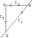
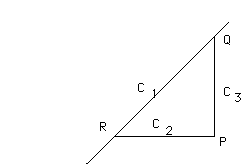
Take the geometry to be as configured in Figure 23.1a or 23.1b with P = {[[alpha]],[[beta]]}, Q = {[[alpha]],[[alpha]]} and R = {[[beta]],[[beta]]}.
Figure 23.1
Then, because dy = 0 on C2 and dx= 0 on C3,
òòD[Ux + Vy] dx dy = I(C1, , )(U dy - V dx) - I(C2, , )V dx + I(C3, , )U dy. (23.7)
From the definition of V in (23.5)
I(C2, , )V dx = I(C2, , )vb u dx + I(C2, , )vux dx. (23.8)
Using integration by parts,
I(C2, , )vux dx = v(P)u(P) - v(R)u(R) - I(C2, , )vx u dx. (23.9)
Hence
I(C2, , )V dx = v(P)u(P) - v(R)u(R) + I(C2, , )(vb-vx) u dx. (23.10)
Pulling together (23.6), (23.7), (23.8), and (23.10), it follows that
òòD [v L[u] - M[v] u] dx dy =
v(P) u(P) - v(R) u(R) + I(C2, , ) (vb-vx) u dx + (23.11)
I(C3, , ) (va - vy) u dy + I(C1, , )(Udy - V dx).
The Riemann Method for solving (23.1) is to find a function v such that
M[v] = 0,
vx = vb on C2,
vy = va on C3,
and v = 1 at {[[alpha]],[[beta]]}.
Such a function is called the Riemann function. If one had such a function, we would have from (23.11) that any u that satisfies L[u] = 0 also satisfies
u(P) = v(R) u(R) - I(C1, , )[Udy - Vdx]. (23.12)
Also, the fundamental theorem of calculus gives the identity
v(R)u(R) - v(Q) u(Q) = I(C1, , ) d[v u] = I(C1, , )[(vu)x dx + (vu)y dy] (23.13)
This may be used with (23.12) to get
u(P) = v(Q)u(Q) + I(C1, , )[(vu)x dx + (vu)y dy] - I(C1, , )[Udy - Vdx]. (23.14)
Hence, combining (23.12) and (23.14),
2 U(P) = u(R) v(R) + u(Q)v(Q) - 2 I(C1, , )[Udy - Vdx]
+ I(C1, , )[(uv)x dx + (uv)y dy] (23.15)
Using the definitions of U and V in (23.14), we simplify:
2 I(C1, , )[Udy - Vdx] = I(C1, , )2vau dy - 2vy u dy - 2vbu dx - 2vux dx (23.16)
and
I(C1, , )[(uv)x dx + (uv)y dy] = I(C1, , )vyu dy + v uy dy + vux dx + vxu dx. (23.17)
Add these and combine with (23.5) to get
u(P) = F(1,2)[v(R)u(R) + v(Q)u(Q)] + I(C1, , )v[a dy - b dx]u +
F(1,2) I(C1, , )v [ uy dy - ux dx] + F(1,2) I(C1, , )[vx dx - vydy] u. (23.18)
which is the solution of the Cauchy problem in terms of the Cauchy data and the Riemann function along the initial curve C1.
Note that the derivative in the direction of the normal is
F([[partialdiff]]u,[[partialdiff]][[eta]]) = {F([[partialdiff]]u,[[partialdiff]]x), F([[partialdiff]]u,[[partialdiff]]y)} {-1,1} = - F([[partialdiff]]u,[[partialdiff]]x) + F([[partialdiff]]u,[[partialdiff]]y).
Hence,
I(Q,R, )v [ uy dy - ux dx] = I(Q,R, )v F([[partialdiff]]u,[[partialdiff]][[eta]]) ds (23.19)
Consider now the problem uxy + ku = 0 with u = f and ux - uy = g on the curve x = y. The Riemann function must satisfy
vxy + kv = 0,
vx = bv where y = [[beta]], (23.20)
vy = av where x = [[alpha]],
and v = 1 at {[[alpha]],[[beta]]}.
Consider v(x,y) = J0(2 R(k(x-[[alpha]])(y-[[beta]]))). We have established that it satisfies the partial differential equation. Recalling that J0(0) = 1, J0' = J1 and that J1(0) = 0, we have the following:
u([[alpha]],[[beta]]) = F(1,2) [f([[alpha]])+f([[beta]])] + F(1,2)I([[beta]],[[alpha]], )J0(2R(k(s-[[alpha]])(s-[[beta]])) ) g(s) ds +
F(1,2)I([[beta]],[[alpha]], )F(R(k)([[alpha]]-[[beta]]),R((s-[[alpha]])(s-[[beta]]))) J1(2R(k(s-[[alpha]])(s-[[beta]])) ) g(s) ds. (23.21)
To get u(x,y), recall that [[alpha]] = x + t and [[beta]] = x - t.
WORK IN PROGRESS:
Add a nonhomogeneous term to (23.1).
What changes if a, b, and c are not constant?
Make equations and graphs solved by this method so that one in convinced
that this method will solve constant coefficient problems.
APPENDIX WITH MAPLE:
Worksheets, And Answers