Linear Methods of Applied Mathematics

Evans M. Harrell II and James V. Herod*

*(c) Copyright 1994,1997,2000 by Evans M. Harrell II and James V. Herod. All rights reserved.

XV. Ordinary differential operators

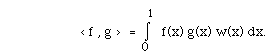
Recall that L²[0,1] is an inner product space when we provide it with the "usual" inner product. You should also recall there are many choices that can be made for an inner product for the functions on [0,1]. One might have a weighted inner product such as we had in Rⁿ and as was described in an appendix to Chapter II. That is, if w(x) is a continuous, non-negative function, we might have

The choices for w(x) are usually suggested by the context in which the space arises.

Some inner product spaces are called Hilbert spaces.

Definition XV.1. A Hilbert space is a vector space on which there is an inner product and on which there is one more bit of structure: It is a complete inner product space, in the sense that if f_p is an infinite sequence of vectors in the space which is Cauchy convergent - meaning that

lim_n,m < f_n-f_m , f_n-f_m > = lim_n,m | f_n-f_m |² = 0

- then there is a vector g, also in the space, such that lim_n f_n = g.

Take this opportunity to review the subject of inner-product spaces in chapter II or follow this link for two examples illustrating the notion of convergence in the Riesz representation theorems cast light on the nature of continuous linear transformations on function space. You may recall that in Rⁿ, if L is a linear function from Rⁿ to R then there is a vector v in Rⁿ such that L(x) = < x, v > for each x in Rⁿ. (More description of the analogue of Riesz representation for Rⁿ.)

In general, where the vector space is not Rⁿ, more is required.

Theorem XV.2. (The Riesz representation theorem for Hilbert space.) If {E, < , >} is a Hilbert space, then these are equivalent:

(a) L is a continuous, linear function from E to R (or the complex numbers C), and

(b) there is a unique member v of E such that L(x) = < x, v > for each x in E.

It is not hard to show that (b) implies (a). To show that (a) implies (b) is more interesting. The argument uses the fact that E is complete and can be found in any introduction to Hilbert space or functional analysis, or this link.

Example XV.3. Since the space of continuous functions on [0,1], denoted C[O,1], with the usual inner product is not a Hilbert space, one should expect that there might be a linear function L from C[0,1] to R for which there is no v in C[0,1] such that

for each f in C[0,1]. In fact, here is such an L:

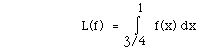
Let

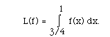
The candidate for v is v(x) =1 on [3/4, 1] and 0 on [0, 3/4). But this v is not continuous! It is only piecewise continuous.

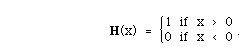
Definition XV.4. The Heaviside function H is defined as follows:

                            (15.1)

Note that

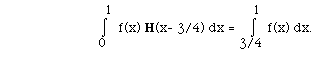
Thus, the Heaviside function provides an element v for which the linear function

has a Riesz representation. As noted, v is not in C[0,1].

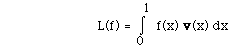
It is not always possible to have a piecewise continuous v which will rectify the situation. Consider the following linear function: L(f) = f(1/2). It is not so hard to see that there is no piecewise continuous function v on [0,1] having the property that for every continuous f,

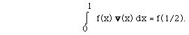
Definition XV.5. The symbol is used to denote the "generalized" function which has the property that

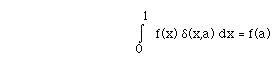                            (15.2)

for some suitably large class of functions f, when 0 < a < 1. It is no surprise that some effort has been made to develop a theory of generalized functions in which the delta function can be found. Generalized functions are also called "distributions". While the delta function is not a well-defined function of the familiar type, it can be manipulated like a function in most cases, provided that in the end it will be integrated, and that the other quantities in the integral with it will be continuous.

A suggestive analogy is that of complex numbers. Like complex numbers, generalized functions are idealizations which do not describe real, physical things, but they have been found tremendously useful in applied mathematics. Most famously they were used by Dirac in his quantum mechanics; it is less well known that mathematical physicist Kirchhoff used them decades earlier in his work on optics. The theory of distributions is attractive and establishes a precise basis for the ideas which these notes will use.

As it turns out, Riesz also provided the essential tool for defining generalized functions:

Definition XV.6. We define some useful function spaces on an arbitrary open set in Rⁿ as follows:

C[] is the set of bounded, continuous functions on .

C_c[] is the subset of C[] consisting of functions which are equal to zero outside some closed, bounded region in . (You may recall that a closed, bounded set in Rⁿ is called compact.)

C_c [] is the set of functions f in C_c[] such that all derivatives of f are also in C_c[]. These are also known as test functions.

The uniform sense of convergence is appropriate for these spaces: Any uniform limit of continuous functions on a fixed bounded set is a continuous function. When we say that a sequence of test functions converges, we mean that the set where the sequence differs from zero is contained in a fixed, bounded region, and not only does the sequence f_k(x) converge uniformly, but so do all of its derivatives. It sounds like a lot to ask for a function to be a test function, and you may even be suspicious that there aren't too many of them. However, it is known that any L² function can be approximated in the r.m.s. sence by test functions, though not in generally in the uniform sense.

Theorem XV.7. (The Riesz-Markov representation theorem.) Suppose that T[f] is a continuous linear functional on the set of test functions C_c [] and is positive in the sense that for any positive test function f(x), T[f] 0. Then T[f] may be considered as an integral, formally written as

The same theorem is true with C_c in place of C_c. We shall return to the delta function when its properties are needed to understand how to construct Green functions.

Differential operators and their adjoints

As suggested in the previous two chapters, the role of the adjoint of a linear function will be critical. If L is a linear function that is defined on some subspace of E, then the task of finding the adjoint L* will involve finding not only how the adjoint is defined, but also what is the subspace composing the domain of definition of L*.

In linear algebra, the adjoint of a square matrix is given by its transpose (if necessary also taking the conugate of any matrix entries which are complex numbers). How can the adjoint be defined for general linear operators?

Definition XV.8. Suppose that L is a continuous linear operator on a Hilbert space. Its adjoint L* is the unique linear operator such that for all f, g,

. If they were, it would be possible to differentiate every square-integrable function and get another square-integrable function, but that is clearly false. Therefore we need to think about the set of functions on which the operator is defined, which is often smaller than the whole Hilbert space. We call this the domain of definition of the operator.

adjoint Definition XV.9. Suppose that L is a linear operator defined on a subspace M of a Hilbert space. The adjoint domain M* is the set of vectors f in the Hilbert space such that for all g in M, the linear functional

_g[f] := <f,Lg> is continuous. The adjoint operator L* is the operator on M* such that <f, Lg> = <L* f, g>.             (15.3) The Riesz representation theorem guarantees that L*f is a uniquely defined vector in H.

A differential operator is not really defined until we specify its domain of definition, and the issue of finding the domain can be technically quite involved. Usually there are two parts sorts of questions about the domain, one having to do with precisely how differentiable the functions must be (which leads into some advanced theory about regularity of functions), and the other having to do with boundary conditions. That is, how can you restrict the functions in M to make sure that when you integrate by parts in order get (15.3), there are no boundary contributions.

In what follows, we shall ignore the question of regularity and discuss only the boundary conditions when we spell out domains of definition of operators.

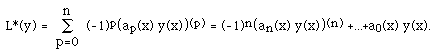
Consider the differential operator L given by

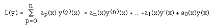
We can define the formal adjoint L* of L by

                            (15.4)

The formal adjoint is exactly what you get when you integrate by parts enough times to obtain the formula (15.3) if you ignore all boundary terms. The second order operator L(y) = a₂(x) y''(x) + a₁(x) y'(x) + a₀(x) y(x), according to this formula, will have formal adjoint

L*(y) = (a₂(x) y(x))'' - (a₁(x) y(x))' + a₀(x) y(x).

If L is not defined on all of E, but just some subspace, or manifold M, then one must find where L* is defined. We denote the domain of L* by M*.

As remarked abovee, The TRUE adjoint L* has to satisfy (15.3), which for a differential operator on the interval [0,1] reads:

                            (15.5)

for all u in M and v in M*. It is often useful to use the following identity resulting from integration by parts:

The important part of finding the adjoint domain M* is to choose conditions on v so that the boundary contributions in formulae like this drop out.

Model Problem XV.10. Let L = D² + 3 x D + x² 1. That is, L(u) = u''(x) + 3x u'(x) + x² u(x). Let us specify that the operator L is defined on the manifold consisting of all regular functions u on [0,1] which satisfy u(0) = u'(1) and u(1) = u'(0). Thus:

M = {u:u(0) = u'(1), u(1) = u'(0)}. Find L* and M*.

Solution. L* will have the form of the formal adjoint:

L*(v) = v'' - (3x v(x))' + x²v(x).

The manifold M* is chosen to make the equation

< L(u), v> = < u, L*(v) >

satisfied.

Since u is in M, u'(1) = u(0) and u(1) = u'(0), so that

< L(u), v > - < u, L*(v) > = [v(1) + v'(0)]u(0) - v'(1) + v(0) - 3v(1)] u'(0).

In order for this last line to be zero for all u in M, the manifold M* should consist of functions f such that

v(1) + v'(0) = 0 and v'(1) + v(0) = 3v(1).

                                                                            QED

These examples introduce the types of problems that we shall consider. We shall provide a method to get solutions for ordinary differential equations with boundary conditions. The problem, together with the boundary conditions, defines the operator L and a manifold M.

Model Problem XV.11.

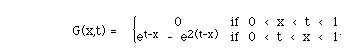
The boundary-value problem y''+ 3y' + 2y = f , y(0) = y'(0) = 0 leads to an operator L and a manifold M given by

L := D² + 3 D + 2 1, and M := {y: y(0) = y'(0) = 0 }. The problem is to solve the following equation: given a continuous function f, find y in M such that L(y) = f. The technique is to construct a function G such that u is given by

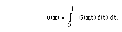
For such problems, we will have techniques to construct G. In this case

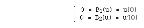
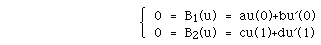
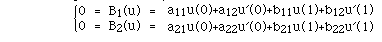
Most frequently, we will consider three types of boundary conditions illustrated below for a second order problem:

Initial conditions

unmixed, two point boundary conditions

mixed, two point boundary conditions

---

The Fredholm alternative theorems for ordinary differential operators.

Before developing a technique for solving these ordinary differential equations with boundary conditions, attention should be paid to the statement of the Fredholm Alternative Theorems in this setting. You may wish to compare it with the alternative theorems for integral equations and for matrices.

Theorem XV.12. Suppose that L is an n^th order differentiable operator with n boundary conditions. B₁, B₂, ...B_n. The problem is posed as follows: Given f, find u such that L(u) = f with B_p(u) = 0, p = 1, 2, ...n.

I. Exactly one of the following two alternatives holds:

(a)(First Alternative) if f is continuous then L(u) = f, B_p(u) = 0, p = 1, 2, ..., n, has one and only one solution..

(b)(Second Alternative) L(u) = 0, B_p(u) = 0, p = 1, 2, ...n, has a nontrivial solution.

II. (a) If L(u) = f, B_p(u) = 0, p = 1, 2, ...n, has exactly one solution then so does L*(u) = f, B_p*(u) = 0, p = 1, 2, ...n have exactly one solution.

(b) L(u) = 0, B_p(u) = 0, p = 1, 2, ... n, has the same number of linearly independent solutions as L*(u) = 0, B_p*(u) = 0, p = 1, 2, ...n.

III. Suppose the second alternative holds. Then L(u) = f, B_p(u) = 0, p = 1, 2, ...n has a solution if and only if < f, w > = 0 for each w that is a solution for
   L*(w) = 0, B_p*(w) = 0, p = 1, 2, ...n.

---

Weak solutions of differential equations

Another use of the representation theorems is to allow us to solve differential equations with solutions which cannot be properly differentiated. Reasons you might want to do this include:

to model phenomena like shock waves

to be able to solve differential equations involving generalized functions like the delta function.

The basic idea is that if f is a test function which satisfies an equation of the form L f = g, Then for all test functions (x), it will be true that <Lf,> = <f, L*> = <g, >             (15.6) Conversely, if (15.6) holds for all possible test functions , and f is also sufficiently regular to allow integration by parts, then we know that L f = g. (Boundary terms do not arise because the test functions zero them all out.)

This means that we can tell that L f = g without directly differentiating f. hence, even if f is not differentiable, we can say that in a certain sense, L f = g:

Definition XV.13. A generalized function f solves

L f = g weakly on a set provided that (15.6) holds for all test functions on .

Notice that although we have been talking about ordinary differential equations, this definition is meaningful for partial differential equations, or, for that matter, equations which involve other operations besides differentiation.

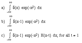
Examples XV.14.

1. For = R, dH(x)/dx = (x).
2. H(x + 2 t) is a weak solution of the equation 2 u/x - u/ t = 0.
3. For = R², H(x-t) is a weak solution of the wave equation u_tt - u_xx = 0. This represents a wave traveling to the right at unit speed.
4. For = R², H(x+t) is a weak solution of the wave equation u_tt - u_xx = 0. This represents a wave traveling to the left at unit speed.

Actually, the previous three examples work for any function h of a single variable in place of the Heaviside function H. We leave the verification of these equations to the Exercises.

---

Exercises XV

XV.1.   Calculate the following integrals:

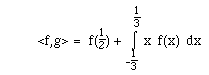
XV.2.   Let <f,g> denote the standard inner product for 0 <= x <= 1.

Find a generalized function g(x) such that

XV.3.   Compute the formal adjoint for each of the following:

(a) L(y) = x² y'' + x y' + y (b) L(y) = y'' + 9 ² y

(c) L(y) = (e^x y'(x))' + 7 y(x) (d) L(y) = y'' + 3y' + 2y

XV.4.   Argue that L is formally self adjoint if it has constant coefficients and derivatives of even order only.

XV.5.   Suppose that L(y) = y'' + 3y' + 2y and y(0)= y'(0) = 0.

Find conditions on v which assure that

XV.6.   Let L(u) = u'' + u. The formal adjoint of L is given by L*(v) = v''+ v. For each manifold M given below, find M* such that L* on M* is the adjoint of L on M.

(a) M = {u: u(0)=u(1)=0},

(b) M = {u: u(0)=u'(0)=0}

(c) M = {u: u(0)+3u'(0)=0, u(1)-5u'(1)=0},

(d) M = {u: u(0)=u(1), u'(0)=u'(1) }.

       (Answers)

XV.7.   Let L and M be as given below; find L* and M*.

(a) L(u)(x) = u''(x) + b(x) u'(x) + c(x) u(x),

M = {u: u(0)=u'(1), u(1) = u'(0) }.

(b) L(u)(x) = -(p(x) u'(x))' + q(x) u(x);

M = {u: u(0) = u(1), u'(0) =u'(1) }.

       (Hint) (c) L(u)(x) = u''(x);

M = {u: u(0) + u(1) = 0, u'(0) - u'(1) = 0 }

       (Answers)

XV.8.   Verify that for L, M, and u as given in Model Problem XV.11, u is in M and L(u) = f. (Recall Exercise 3 in the introduction to the problems of Green functions.)

Suppose G is as in Model Problem XV.11, and

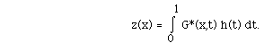
Show that z solves L* z = h for z in M*.

XV.9.   Decide whether the following operators L are formally self adjoint, and whether they are self adjoint on M. Decide whether the equation L(y) = f on M is in the first or second alternative.

(a) L(y) = y'', M = {y: y(0) = y'(0) = 0 }.
       (Answer)

(b) L(y) = y'', M= {y: y(0) = y(1) = 0 }.
       (Answer)

(c) L(y) = y'' + 4 ²y, M={y: y(0) = y(1), y'(0) = y'(1)}.
       (Answer)

(d) L(y) = y'' + 3y' + 2y, M = {y: y(0) = y(1) = 0}.
       (Answer)

XV.10.   Suppose that L(y)(x) = y''(x) + 4 ²y(x). B₁(y) = y(0) and B₂(y) = y(1).

(a) Show that the problem L(y) = 0, B₁(y)= B₂(y) = 0 has sin(2 x) as a non-trivial solution.

(b) What is the adjoint problem for {L, B₁, B₂}?

(c) What specific conditions must be satisfied by f in order that L(y) = f, y(0) = 0 = y(1) has a solution?

(d) Show that y''(x) + 4 ²y(x) = 1, y(0) = 0 = y(1) has

[ 1 - cos(2 x) ] /4 ² as a solution.

XV.11.   Show that y'' = x, y'(0) = 0 = y'(1) has no solution.

XV.12.   Show that y'' = sin(2 x), y'(0) = 0 = y'(1) has a solution.

XV.13.   Verify that the differential equations in Examples XV.14 have the weak solutions stated there.
Hint for the wave equation. Change variables to r = x+t and s = x-t.

---

Link to

Chapter XIV (beginning) (second part)

chapter XVI

Table of Contents

Evans Harrell's home page

Jim Herod's home page